
Logistic Regression and the Incidental Parameters Problem
Published:
This is the first in a series of posts in which I’ll discuss basic issues in econometric analysis, and common pitfalls. I will demonstrate the issues intuitively, and concretely, via simulation. Hopefully by providing this code, anyone who comes across the material can see and play with it themselves to better understand the issues. All simulations will be conducted in R.
Incidental Parameters Problem
The incidental parameters problem (henceforth IPP) is a well-known problem in econometrics, dating back more than 80 years. The seminal paper introducing the problem was published by Jerzy Neyman and Betty Scott in Econometrica in 1948. I won’t rehash the details of the issue here, but I’ll give you the punch line.
With linear regression, we generally address time invariant confounds in panel data via fixed effects (either panel dummies, or the mathematically equivalent within-transformation).
Unfortunately, those methods do not ‘work’ in non-linear regression, because the fixed effects enter the specification multiplicatively (the only exception here is Poisson regression, where the math still works out as a matter of convenience).
Fortunately, Gary Chamberlain derived conditional logit, wherein the panel fixed effects are instead addressed via a transformation to the likelihood function.
While I encourage anyone to go and read these papers, my goal here is to demonstrate concretely, via simulation, just how poorly a dummy fixed effect estimator performs in the case of panel logistic regression. I will first simulate a simple scenario of static confounding, wherein a standard logistic regression model fails to recover the parameter of interest. I will then compare its performance against alternative correction procedures, namely a dummy fixed effect estimator and the Chamberlain conditional logit estimator. Notably a more recent literature pursues bias correction methods for general non-linear panel data models, e.g., Fernandez-Val (2009) in the Journal of Econometrics. I will thus also explore the efficacy of Fernandez-Val’s bias correction following dummy fixed effect logit.
Simulation Setup
The simulation setup is as follows. I begin with 100 panel units and simulate a time-invariant characteristic that serves as the confound. I then combine the units into a data frame.
# I begin by setting some simulation parameters.
set.seed(2040)
n <- 100
sims <- 100
panel_max <- 10

# Lastly, for each panel unit
confound <- rnorm(n, mean = 0, sd=1)
id <- seq(n)
treatment_grp <- rbinom(n=n, size=1, prob=confound > median(confound))
df <- data.frame(confound=confound,id = id, treatment_grp = treatment_grp)
In each run of the simulation, I create a new panel data set, extending off the basic setup. I expand the original data-frame into repeated observations of each panel, to varying lengths, T = 2..10. With each new panel dataset, I turn the treatment ‘on’ for the treatment group at the panel midpoint (rounded down).
After I create a dataset, I estimate four alternative logistic regression models:
- A naive regression (ignoring the confound)
- A dummy fixed effect regression (the incidental parameters problem applies here)
- A dummy fixed effect regression with analytical correction (using the ‘bife’ package)
- A conditional logit regression (this is the idea approach)
- An oracle regression (standard logit, conditioning on the confound)
# I create an empty data frame to store all the simulation results, based on the simulation paramters
sim_result <- expand.grid(periods = seq(from=2,to=panel_max,by=1),run = seq(sims))

# Simulate each panel length 100 times and re-run all models.
for (r in 1:sims){
  for (p in seq(from=2,to=panel_max,by=1)){

      # Simulate a panel of p periods.
      # Make the data with whole panel length
      df_tmp <- expandRows(df, count=p, count.is.col=FALSE)

      # Treatment begins midway through the panel for treated units.
      df_tmp <- df_tmp %>% group_by(id) %>% mutate(period = seq(from=1,to=p,by=1)) %>% mutate(Treat = (period > floor((p+1)/2))*treatment_grp) %>% arrange(treatment_grp,id,period) %>% select(-c(treatment_grp))
      df_tmp$Treat_center <- df_tmp$Treat - mean(df_tmp$Treat)
      df_tmp$xb <- 2*df_tmp$Treat_center + 4*df_tmp$confound
      df_tmp$p <- inv.logit(df_tmp$xb)
      df_tmp$Y <- rbinom(nrow(df_tmp),size=1, prob=df_tmp$p)

      # Estimate our four logit models.
      logit_mod_control <- glm(data=df_tmp,Y ~ Treat_center + confound, family = "binomial")
      logit_mod_omit <- glm(data=df_tmp,Y ~ Treat_center, family = "binomial")
      logit_mod_fe <- clogit(data=df_tmp,Y ~ Treat_center + strata(id))
      logit_mod_ipp <- glm(data=df_tmp,Y ~ Treat_center + factor(id), family = "binomial")

      # Sometimes the analytical correction fails, and it doesn't handle it well.
      tryCatch(
        {
          # Let's set a placeholder result to NA in case the estimation fails.
          logit_mod_bife <- data.frame(coefficients=NA)
          suppressWarnings(logit_mod_bife <- bias_corr(bife(Y~Treat_center | id,data=df_tmp)))
        },error=function(cond){
          # BIFE crapped out.
          return(logit_mod_bife)
        },warning=function(cond){
          # BIFE generated a warning.
          return(logit_mod_bife)
        }
      )

      sim_result_row <- data.frame(cbind(periods=p,run=r,b_control=logit_mod_control$coefficients[2],b_omit=logit_mod_omit$coefficients[2],b_fe=logit_mod_fe$coefficients[1],b_ipp=logit_mod_ipp$coefficients[2],b_bife=logit_mod_bife$coefficients[1]))

      sim_result <- sim_result %>% left_join(sim_result_row,by=c("periods","run"))
      sim_result$b_control.y[is.na(sim_result$b_control.y) ] <- sim_result$b_control.x[ is.na(sim_result$b_control.y)]
      sim_result$b_omit.y[is.na(sim_result$b_omit.y) ] <- sim_result$b_omit.x[ is.na(sim_result$b_omit.y)]
      sim_result$b_fe.y[is.na(sim_result$b_fe.y) ] <- sim_result$b_fe.x[ is.na(sim_result$b_fe.y)]
      sim_result$b_ipp.y[is.na(sim_result$b_ipp.y) ] <- sim_result$b_ipp.x[ is.na(sim_result$b_ipp.y)]
      sim_result$b_bife.y[is.na(sim_result$b_bife.y) ] <- sim_result$b_bife.x[ is.na(sim_result$b_bife.y)]

      if("b_control.y" %in% colnames(sim_result)){
        sim_result <- sim_result %>% select(-c(b_control.x, b_omit.x, b_fe.x, b_ipp.x,b_bife.x)) %>% rename(b_control=b_control.y, b_omit = b_omit.y, b_fe = b_fe.y, b_ipp = b_ipp.y, b_bife = b_bife.y)
      }
   }
}
Regression Output
Let’s take a quick look at the output from the final set of regressions, in the last iteration. Note that I am omitting the intercept and dummy coefficients in the output.
screenreg(list(logit_mod_omit,logit_mod_ipp,logit_mod_bife,logit_mod_fe,logit_mod_control),
          digits=3,omit.coef=c("factor|Intercept|confound"),
          custom.model.names=c("logit","logit + dummies","bife","clogit","logit + control"))
##
## ==========================================================================================
##                 logit         logit + dummies  bife          clogit        logit + control
## ------------------------------------------------------------------------------------------
## Treat_center       3.481 ***     1.551 ***        1.391 ***     1.394 ***     1.618 ***
##                   (0.277)       (0.363)          (0.354)       (0.343)       (0.323)
## ------------------------------------------------------------------------------------------
## AIC             1063.720       594.164                        296.280       471.803
## BIC             1073.536      1089.847                                      486.526
## Log Likelihood  -529.860      -196.082         -196.181                    -232.901
## Deviance        1059.720       392.164          392.362                     465.803
## Num. obs.       1000          1000              440          1000          1000
## R^2                                                             0.019
## Max. R^2                                                        0.269
## Num. events                                                   479
## Missings                                                        0
## ==========================================================================================
## *** p < 0.001; ** p < 0.01; * p < 0.05
Visualizing the Distribution of Estimates
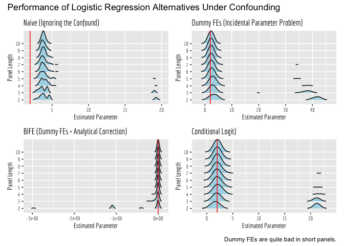
Okay, but how consistently did each alternative estimator perform, across the 100 runs? Let’s visualize this. One thing to note here is that sometimes the estimators fail to converge, and thus spit out woefully inaccurate estimates (off by orders of magnitude). So, we will first look at the general plots, so you can see how often these happen across the different estimators. Then, we will zoom in on the “valid” estimates!
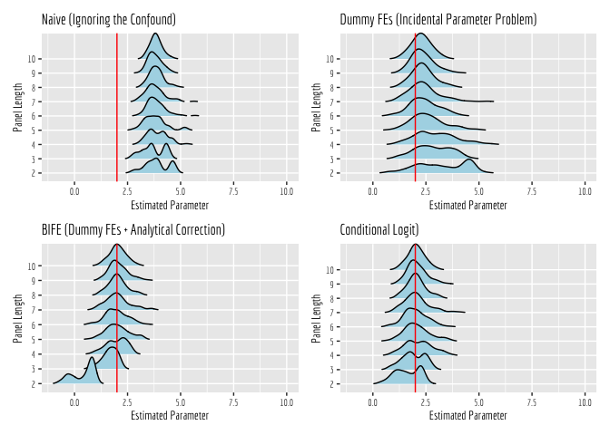
Now we will zoom in around 2, to the estimates that were generated by models that converged. What is pretty apparent here is that the Naive estimator is inconsistent; it is converging to an incorrect value, regardless of panel length. All of the other estimators converge to the correct value, given enough data and sufficiently long panels. However, they clearly do so at different rates.
Most notably, the dummy fixed effect estimator only manages to converge to the correct value when panels get sufficiently long. In short panels, this estimator performs quite poorly. The analytically corrected dummy fixed effect estimator (estimated using the ‘bife’ package) also does poorly in short panels, but it appears to recover more quickly as panel lengths increase. The conditional logit estimator, on the other hand, does well right off the bat, even in short panels!
A couple of final thoughts.
A natural question you might have is “what constitutes a sufficiently long panel?” Well, that is never truly knowable, because it will depend on your sample and context. Accordingly, as a general rule, you should not use dummy fixed effects.
Be careful about convergence; you will notice that all of these estimators frequently fail to converge. When that happens, in many cases, you still get an estimate, but it is meaningless. Be careful to ensure the model converged before you take an estimate and run with it!