Clustered Standard Errors With (Too) Few Clusters

Back in April 2021 I posted a Twitter thread with a small simulation of what happens to cluster-robust standard errors when you only have a handful of clusters. It got passed around more than I expected, and Alexander Fischer (author of the excellent fwildclusterboot package) wrote a nice follow-up that added Satterthwaite-corrected standard errors to the comparison. The thread never made it onto this site, and the original code has aged (it used multiwayvcov, which has since left CRAN). So here is an updated version, with the small-sample corrections folded in.

The problem

We cluster standard errors because observations within a group (a state, a firm, a classroom, a subreddit) share unobserved shocks, so regression errors are correlated within the group. Ignore that and you understate your standard errors, sometimes badly (Moulton, 1986). The standard fix is the cluster-robust “sandwich” variance estimator of Liang and Zeger (1986) (what I will call vanilla cluster SEs), which is consistent as the number of clusters, $G$, goes to infinity.

The catch is that $G$ is frequently not large. Papers cluster on 50 states, on a dozen regions, or on the six sites of a field experiment. Two questions follow: how badly do clustered standard errors perform when $G$ is small, and what can we do about it? The answer to the second question, at least for the linear model, is well developed: use a better small-sample adjustment (Bell and McCaffrey, 2002; Imbens and Kolesár, 2016; Pustejovsky and Tipton, 2018) or use the wild cluster bootstrap (Cameron, Gelbach and Miller, 2008; Roodman et al., 2019). MacKinnon, Nielsen and Webb (2023) is a good current guide to all of this. The point of this post is just to see it.

The data generating process

I simulate a bivariate regression $y = 0.1 + 0.5x + e$ with $n = 1000$ observations split evenly across $G$ clusters. Both the regressor and the error have a cluster-level component:

where the individual-level pieces are independent normal draws and the cluster-level pieces are shared by everyone in cluster $g$. I set the intra-cluster correlation of the error to $\rho = 0.7$ by giving $e^{(g)}$ variance $\rho$ and $e^{(i)}$ variance $1-\rho$. The cluster component of $x$ matters too: the Moulton inflation factor for the standard error scales with the product of the intra-cluster correlations of $x$ and $e$ (and with cluster size), so a clustered error term alone does not do much damage if $x$ varies freely within clusters. Note that $x$ and $e$ are independent, so there is no endogeneity here.

suppressPackageStartupMessages({
  library(dplyr); library(ggplot2); library(patchwork)
  library(sandwich); library(clubSandwich); library(fwildclusterboot); library(future.apply)
})

gen_cluster <- function(n = 1000, G = 50, rho = 0.7, beta = c(0.1, 0.5)) {
  n <- ceiling(n / G) * G                      # balanced clusters
  ind <- mvtnorm::rmvnorm(n, sigma = diag(c(1, 1 - rho)))   # individual parts of (x, e)
  cl  <- mvtnorm::rmvnorm(G, sigma = diag(c(1, rho)))       # cluster parts of (x, e)
  cluster <- rep(seq_len(G), each = n / G)
  x <- ind[, 1] + cl[cluster, 1]
  e <- ind[, 2] + cl[cluster, 2]
  data.frame(x = x, y = beta[1] + beta[2] * x + e, cluster = cluster)
}

4 approaches to constructing cluster SEs

For every simulated dataset I fit lm(y ~ x) once and then construct standard errors using each approach:

1. Regular OLS. The textbook standard error, which assumes independent errors.
2. CR1, $t(n-k)$. Vanilla cluster SEs: the cluster-robust sandwich with Stata’s $\frac{G}{G-1}\frac{n-1}{n-k}$ finite-sample factor, paired with the same critical value OLS would use. This is what R’s sandwich::vcovCL() followed by lmtest::coeftest() gives you by default.
3. CR1, $t(G-1)$. Identical variance estimate, but with critical values from a $t$ distribution with $G-1$ degrees of freedom. This is the default in Stata’s vce(cluster) and in R’s fixest.
4. CR2 + Satterthwaite. The bias-reduced CR2 sandwich of Bell and McCaffrey (2002), with Satterthwaite degrees of freedom, via clubSandwich.
5. Wild cluster bootstrap. 999 bootstrap draws imposing the null, via fwildclusterboot. I use Rademacher weights, switching to Webb’s six-point weights when $G \le 12$, as Roodman et al. (2019) recommend. The confidence interval is obtained by test inversion.

one_sim <- function(G, n = 1000, rho = 0.7, B = 999, seed = 1) {
  set.seed(seed); dqrng::dqset.seed(seed)
  d <- gen_cluster(n = n, G = G, rho = rho)
  fit <- lm(y ~ x, data = d)
  b <- unname(coef(fit)["x"]); n_obs <- nrow(d)

  ci_reg <- confint(fit)["x", ]

  V1  <- sandwich::vcovCL(fit, cluster = ~cluster, type = "HC1")
  se1 <- sqrt(V1["x", "x"])
  ci_cr1_n <- b + c(-1, 1) * qt(0.975, n_obs - 2) * se1
  ci_cr1_g <- b + c(-1, 1) * qt(0.975, G - 1) * se1

  ci_cr2 <- tryCatch({
    ct <- clubSandwich::conf_int(fit, vcov = "CR2", cluster = d$cluster,
                                 test = "Satterthwaite", coefs = "x")
    c(ct$CI_L, ct$CI_U)
  }, error = function(e) c(NA, NA))

  ci_wild <- tryCatch({
    bt <- suppressWarnings(suppressMessages(fwildclusterboot::boottest(
      fit, param = "x", clustid = "cluster", B = B,
      type = if (G <= 12) "webb" else "rademacher")))
    bt$conf_int
  }, error = function(e) c(NA, NA))

  data.frame(G = G, b = b,
             method = c("regular", "cr1_t_n", "cr1_t_g", "cr2_satt", "wild"),
             lo = c(ci_reg[1], ci_cr1_n[1], ci_cr1_g[1], ci_cr2[1], ci_wild[1]),
             hi = c(ci_reg[2], ci_cr1_n[2], ci_cr1_g[2], ci_cr2[2], ci_wild[2]))
}

Running it

I run 1000 replications for every cluster count from 2 to 50.

run_sims <- function(G_grid, n_sims = 1000, n = 1000, rho = 0.7, B = 999,
                     workers = max(1, parallel::detectCores() - 4)) {
  grid <- expand.grid(G = G_grid, sim = seq_len(n_sims))
  plan(multisession, workers = workers); on.exit(plan(sequential), add = TRUE)
  res <- future_lapply(seq_len(nrow(grid)), function(i) {
    r <- one_sim(G = grid$G[i], n = n, rho = rho, B = B, seed = 1e6 + i)
    r$sim <- grid$sim[i]
    r
  }, future.seed = TRUE)
  bind_rows(res)
}

sims <- run_sims(G_grid = 2:50) %>%
  mutate(covered = lo <= 0.5 & hi >= 0.5,
         method = factor(method, levels = c("regular", "cr1_t_n", "cr1_t_g", "cr2_satt", "wild"),
                         labels = c("Regular OLS", "CR1, t(n-k): R sandwich + coeftest default", "CR1, t(G-1): Stata / R fixest default",
                                    "Clustered CR2 + Satterthwaite", "Wild cluster bootstrap")))

coverage <- sims %>%
  group_by(G, method) %>%
  summarise(coverage = mean(covered, na.rm = TRUE),      # coverage among intervals that were produced
            failed = mean(is.na(covered)),               # share of replications with no interval (bootstrap only)
            med_width = median(hi - lo, na.rm = TRUE), .groups = "drop")

Vanilla clustering with a sufficiently large number of clusters

Start with $G = 50$. The top panel uses regular OLS standard errors; the bottom uses vanilla cluster SEs. Each point in the plot reflects one point estimate from a single simulated dataset. Red points are those where the 95% CI does not include the true value of 0.5 I specified in my data-generating process.

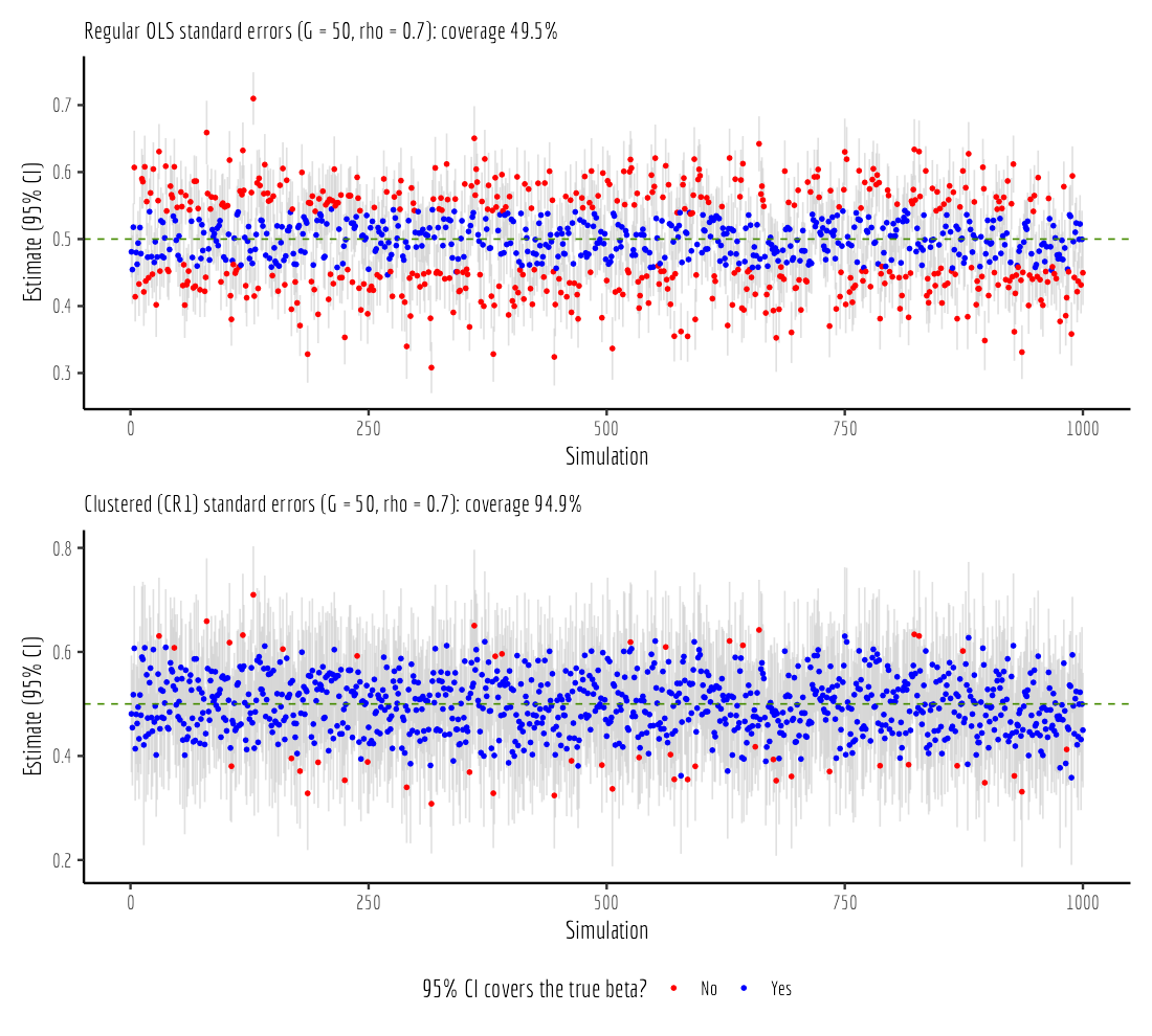
With regular standard errors the “95%” interval covers the truth 49.5% of the time. The estimates themselves are unbiased but the 95% CI is too narrow. Clustering fixes most of the problem: coverage rises to 94.9%.

Six clusters

What happens when we cut $G$ from 50 to 6? Each cluster now has about 167 observations. The top panel uses vanilla cluster SEs; the bottom the wild cluster bootstrap.

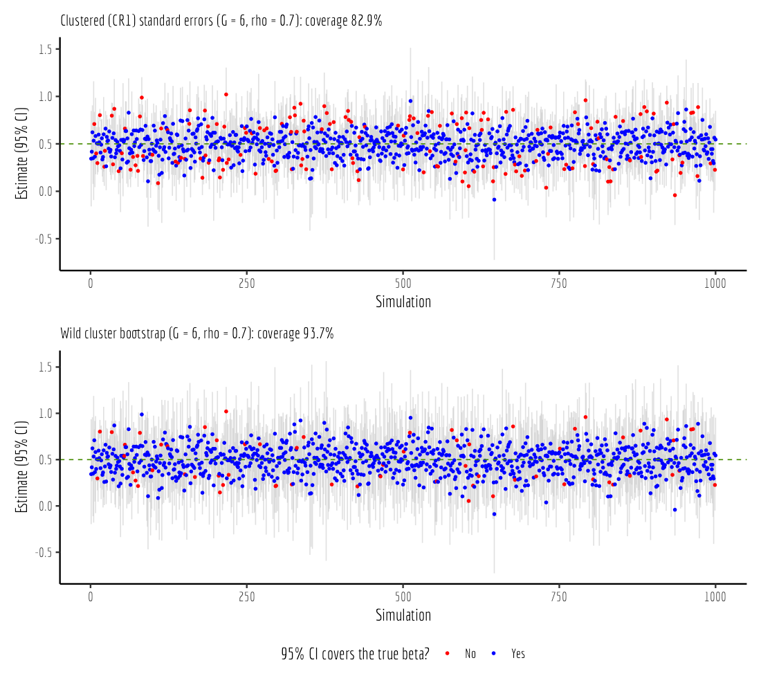
With six clusters vanilla cluster SEs cover the truth only 82.9% of the time; regular standard errors are hopeless at 18.8%. The wild cluster bootstrap gets to 93.7%. Its intervals are somewhat wider and more variable in width.

Coverage as a function of the number of clusters

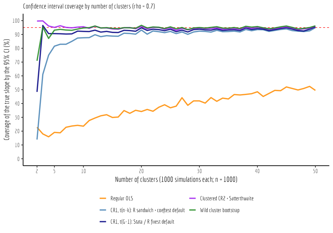
Here is the full picture, for every $G$ from 2 to 50 and all five procedures.

Coverage (%) of nominal 95% confidence intervals.

A few things stand out.

1. Regular standard errors get worse as clusters get fewer. With $n$ fixed, fewer clusters means bigger clusters, and the Moulton factor grows with cluster size. At $G = 2$ coverage is 22.8%; even at $G = 50$ it is only 49.5%.
2. Vanilla cluster SEs undercover below 30 or so clusters, and badly below 10. At $G = 10$ it covers 87.6%; at $G = 5$, 81.5%.
3. Using $t(G-1)$ critical values is free and helps. Same variance estimate, coverage of 92.2% at $G = 10$ and 90.6% at $G = 5$. If your software does this by default (Stata and fixest do), you are already better off than the 2021 thread was.
4. CR2 with Satterthwaite degrees of freedom and the wild cluster bootstrap are both close to nominal down to about five clusters. At $G = 6$ they cover 96.3% and 93.7% respectively. Alexander’s horse race reached the same conclusion, and there is no strong reason to prefer one over the other in a design this simple. CR2’s cost grows with cluster size (it takes a matrix square root per cluster), the bootstrap’s with the number of draws; the bootstrap generalises more easily to awkward settings (wildly different cluster sizes, few treated clusters, and so on; see MacKinnon and Webb, 2017, and MacKinnon, Nielsen and Webb, 2023).
5. Below five clusters, the picture is erratic and no procedure is comfortable. With two clusters the wild bootstrap fails to return an interval at all in 60% of replications (Webb weights give only $6^G = 36$ distinct draws) and covers 70.9% when it does. CR2 with Satterthwaite goes the other way: the degrees of freedom collapse toward one, the median interval is 1.04 wide (the slope is 0.5), and coverage is 99.7%. At three and four clusters the corrections are back in the neighbourhood of nominal, but with intervals two to four times as wide as at ten clusters. None of that is a defect of the methods. Two or three clusters means two or three independent observations of the cluster-level shock, and an honest procedure will tell you so, either by failing or by handing you an interval that spans everything.

Takeaways

If you cluster, know how many clusters you have. Above 40 or 50, vanilla cluster SEs are fine. Between roughly 10 and 40, at minimum use $t(G-1)$ critical values, and preferably CR2 or the wild cluster bootstrap. Below 10, use CR2 or the bootstrap and report the interval, not just the stars. And below five, be honest with yourself and your readers that the data cannot tell you much about sampling variability at the cluster level.

The original 2021 code is archived in this repository; the version above supersedes it. Alexander Fischer’s extended simulations, including unbalanced cluster sizes and the few-treated-clusters case, are in his clusteredErrorsSims package.